The Fractal Generator.

By Theo Fabi & Max Brodeur

December 2021

Overview

This research project was an optional part of the MATH326 - Nonlinear Dynamics & Chaos course offered by McGill during the Fall 2021 semester.

Built using Python, HTML and CSS, our Fractal Generator web application includes the following fractal generating functionalities:

  1. Chaos Game: Fractals such as the sierpinski triangle and the viscek square can be drawn using the chaos game feature. The user can choose the initial polygon, specify the compression ratio of each iteration, and incorporate extra rules to form a variety of attractors. The user can also select from a list of attractor presets which load the appropriate parameters for the attractor.
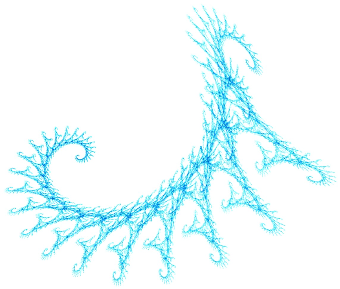
  2. General Iterated Function Systems: The application incorporates the more general concept of iterated function systems (IFSs), with which even more complex fractals can be constructed, wherein the user specifies a list of possible transformation parameters and their relative weights. Presets for the dragon curve, the barnsley fern and other such shapes can be loaded and drawn.
  3. Chaotic Discrete Map generator: 
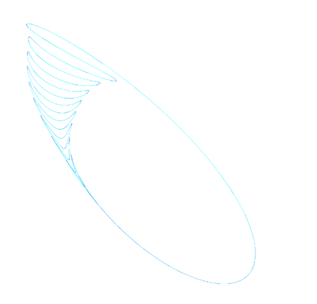
The application has the feature to iteratively find 2D chaotic discrete maps. The details of this functionality will be discussed in detail in Section 3.

Link to fractal generator web application. (Please allow some time for loading the application – it is hosted by the Heroku platform on a free plan.)

Iterated Function System & Chaos Game

An Iterated Function System (IFS) is a finite set of contractive functions which are applied iteratively on an initial point ad infinitum. At every iteration, one transformation among the set is chosen at random and applied to the previous point, yielding the next input for the next iteration. Often, these systems form self-similar fractals, as an arbitrary point at an arbitrary iteration is subject to the same conditions as any other point. In general, it is required that these transformations be contractive, otherwise solutions may be unbounded. However, the general requirement is that the entire system must be contractive on average. 
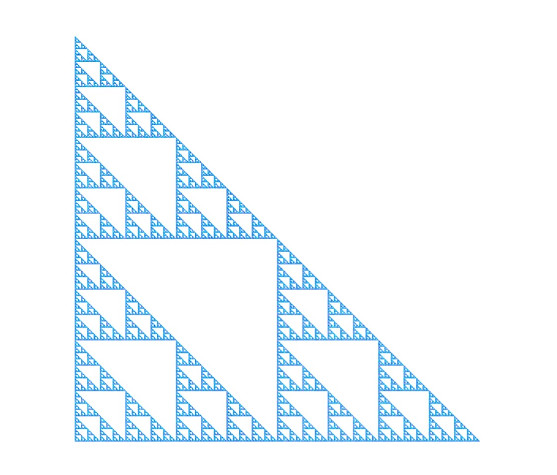
The chaos game is an example of an IFS. In brief, the classical version of the process consists of choosing a random point within an equilateral triangle and repeatedly applying the following procedure:

  1. Randomly choose one of the vertices of the triangle
  2. Jump half-way from the previous point to the chosen vertex
  3. Repeat with the newly drawn point The game can formally be defined as an IFS with the following three choices of transformations:
    • \((x_{n+1}, y_{n+1})= (0.5\;x_n, 0.5 \;y_n)\)
    • \((x_{n+1}, y_{n+1})= (0.5\;x_n + 0.5, 0.5 \;y_n)\)
    • \((x_{n+1}, y_{n+1})= (0.5\;x_n, 0.5 \;y_n + 0.5)\)

After a suficient number of iterations of these transformations, and with initial conditions within the triangle, the Sierpinski right triangle is generated. This is a surprising result given that the transformations are chosen at random. The system consistently forms the same fractal attractor!

The sierpinski right triangle generated with our website.

The IFS Dragon generated with our website.

Other fractals can be constructed using this method. Both the Chaos Game IFS abstraction and general IFS fractal generation features are incoporated in the website. Both of the above fractals can be generated using pre-loaded presets in our web application, along with many others.

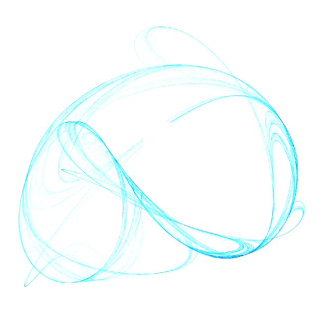
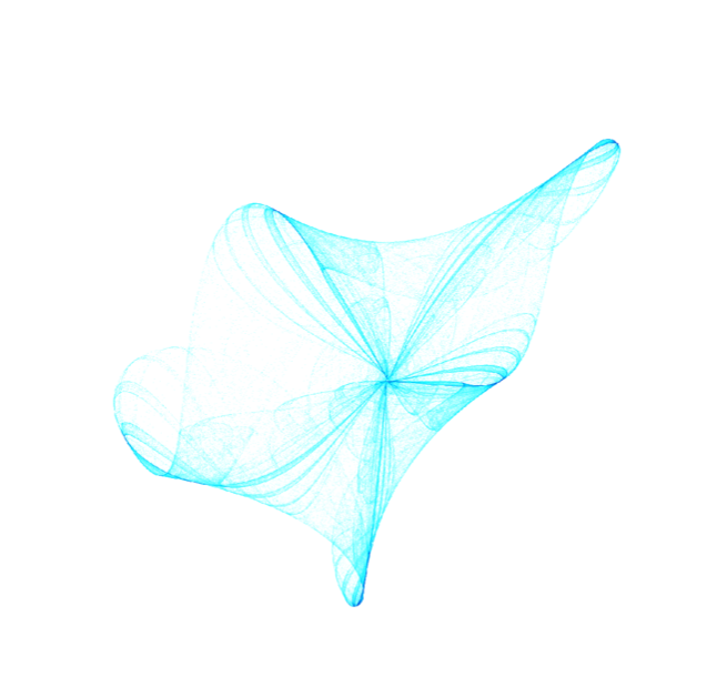
Automatic Generation of Discrete Chaotic Attractors

1D discrete maps can exhibit chaotic behaviour if their lyapunov exponent is positive. Similarly, 2D discrete maps, which have two lyapunov exponents (one for each dimension) exhibit chaotic behaviour if one of their lyapunov exponents is positive. Our website includes a feature which automatically finds quadratic and cubic chaotic 2D maps. When plotted, these systems often yield beautiful fractal shapes. Finding such maps consists of first generating a random map and calculating its lyapunov exponents. If one of them is positive and the map is bounded, it is chaotic. Otherwise, the process shall be repeated until the conditions are satisfied.
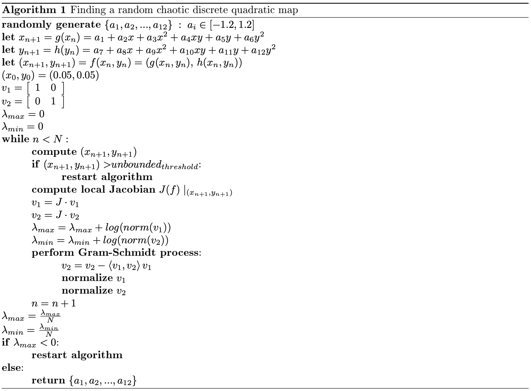
 The following pseudocode demonstrates the logic of the implemented algorithm:

Similar to the pull-back algorithm, the above process is analogous to the classical computation of the lyapunov exponents of a map. However, instead of computing \(\lambda\) in terms of a perturbation \(\delta\), it uses the tangent space map \(J(f)\) and displacement vectors \(v_1\) and \(v_2\). The displacement vectors are orthogonalized after each iteration so as to let each vector align with the corresponding eigendirections/lyapunov directions, and normalized so as to prevent huge computations. It must be noted that the lyapunov exponents are updated before the orthonormalization process. The process is almost identical for cubic maps, but more parameters must be generated.

Silk

Starfish

Wave quasi-cycle

Application Manual

Upon entering the website, the Chaos Game tab is visible. The following parameters are available for editing and manipulation:

Chaos Game parameters hotbar

  • Presets: A list of available attractors which, upon selection, load the appropriate parameters
  • Iterations: The number of points to plot
  • Jump: Compression ratio value (jump distance)
  • Polygon: The number of vertices in the initial shape.
  • Length: The number of previous vertex choices to keep track of for extra rules.
  • Offset: The banned offset from the last chosen vertex when the last n chosen vertices are the same (where n = length)
  • Symmetry: Wether or not the banned offset should be applied to both sides
  • Stack midpoints: Wether or not the midpoints between each vertex can be jumped to
  • Stack center: Wether or not the center of the initial polygon can be jumped to
  • Fast plotting: Wether or not datashading is used for plotting (datashading is much faster, but has a fixed resolution, yielding a less interactive experience)
  • Auto update: Wether or not the fractal should be redrawn when any of the parameters are changed
Rule Description Length Offset Symmetry
The next vertex cannot be 1 vertex awayfrom the last vertex when the last 3 chosen vertices are equal 3 1 True
No extra rules 0 x x
The next vertex cannot be 2 vertices
Away (counterclockwise) as the last vertex 1 2 False
The next vertex can't be the same as the last vertex 1 0 x

The user can also navigate to other sub-sections of our application by interacting with top right corner:

The website's tabs

By default, the Chaos Game tab is selected. If the Transformations tab is selected, the following options are visible when the Parameters dropdown section is activated:

Default Transformations tab parameters

  • Transformation presets: A list of available attractors which, upon selection, load the appropriate parameters
  • Color Presets: Self-explanatory
  • Parsing Type: See Transformations below.
  • Iterations: The number of iterations to plot (Note: since datashading is used, this does not directly correspond to the number of visible points)
  • Transformations: A text area in which the user can specify the possible choices of parameters for the IFS. Every line needs to correspond to one specific transformation choice. The input should follow general CSV file for- matting. Every parameter within a specific transformation choice must be separated by a comma, and every transformation must be separated by a linebreak. In the above example, one of the following two transfor- mations can be chosen at every iteration (with the parameters truncated to two decimal places): \(f_1(x,y) = (0.82\;x + 0.28\;y − 0.21, 0.86\;x − 1.88\;y − 0.11)\) and \(f_2(x, y) = (0.088\;x + 0.52\;y − 0.46, −0.377\;x + 0.78\;y + 8.09)\). The Parsing Type section dictates how the comma-separated parameters are ordered for defining the functions. The Parsing Type option is simply a convenience setting to facilitate copy-pasting parameters from other sources, since some sources may list the parameters in a different order.
  • Probabilities: The relative probabilistic weights of each transformation/set of parameters. In the above example, there is an \(80\%\) chance that \(f_1\) will be chosen, and a \(20\%\) chance that \(f_2\) will be chosen. If the user has supplied n transformations (i.e., there are \(n\) lines in the Transformations input), then n comma-separated values must be entered in the Probabilities section.

If the Random Chaos Finder tab is selected, the following options are visible when the Parameters dropdown section is activated:

Default Random Chaos Finder tab parameters

  • Chaotic Map Order:Wether quadratic or cubic chaotic maps are generated
  • Plot Iterations: The number of iterations in thousands to plot (with datashading)
  • Discard the first \(n\) points when testing: The number of transients, i.e. the number of iterations after which the algorithm should assume the state is within the attractor.
  • Map iterations: The number of test iterations, i.e. the number of iterations the algorithm should use to numerically approximate the lyapunov exponents. In the above example, the lyapunov exponents are calculated over 70,000 iterations. After 70,000 iterations, the program checks wether the largest lyapunov exponent is positive. If it is, the fractal is then plotted with \(n\) iterations, where \(n =\) Plot Iterations. Otherwise, the algorithm is repeated until a satisfactory system is found.
  • Randomization type: Either Continuous or Discrete mode can be selected. If Continous is selected, the random param- eters generated can take any real-valued number within the \([−1.2, 1.2]\) range. If Discrete mode is selected, the random parameters can take value in the \(\{−1.2, −1.1, …, 0, 0.1, …, 1.1, 1.2\;\}\) set. When Find next chaotic map is clicked, the algorithm will run. When a chaotic map is found, it will be drawn and displayed with datashading. In addition, the generated parameters are displayed above the drawn attractor. In Continous mode, the parameters rounded to 4 decimal digits are displayed. In Discrete mode, the parameters are represented as a a string of characters, where \(A\) corresponds to \(-1.2\), \(B\) corresponds to \(-1.1\), and so on.